Even though the title is quite a mouthful, this post is about two really cool ideas:
- A solution to the "chicken-and-egg" problem (known as the Expectation-Maximization method, described by A. Dempster, N. Laird and D. Rubin in 1977), and
- An application of this solution to automatic image clustering by similarity, using Bernoulli Mixture Models.
For the curious, an implementation of the automatic image clustering is shown in the video below. The source code (C#, Windows x86/x64) is also available for download!
Automatic clustering of handwritten digits from MNIST database using Expectation-Maximization algorithm
While automatic image clustering nicely illustrates the E-M algorithm, E-M has been successfully applied in a number of other areas: I have seen it being used for word alignment in automated machine translation, valuation of derivatives in financial models, and gene expression clustering/motif finding in bioinformatics.
As a side note, the notation used in this tutorial closely matches the one used in Christopher M. Bishop's "Pattern Recognition and Machine Learning". This should hopefully encourage you to check out his great book for a broader understanding of E-M, mixture models or machine learning in general.
Alright, let's dive in!
1. Expectation-Maximization Algorithm
Imagine the following situation. You observe some data set  (e.g. a bunch of images). You hypothesize that these images are of
  different objects... but you don't know which images represent which objects.
Let  be a set of latent (hidden) variables, which tell precisely that: which images represent which objects.
Clearly, if you knew , you could group images into the clusters (where each cluster represents an object), and vice versa, if you knew the groupings you could deduce . A classical "chicken-and-egg" problem, and a perfect target for an Expectation-Maximization algorithm.
Here's a general idea of how E-M algorithm tackles it. First of all, all images are assigned to clusters arbitrarily. Then we use this assignment to modify the parameters of the clusters (e.g. we change what object is represented by that cluster) to maximize the clusters' ability to explain the data; after which we re-assign all images to the expected most-likely clusters. Wash, rinse, repeat, until the assignment explains the data well-enough (i.e. images from the same clusters are similar enough).
(Notice the words in bold in the previous paragraph: this is where the expectation and maximization stages in the E-M algorithm come from.)
To formalize (and generalize) this a bit further, say that you have a set of model parameters  (in the example above, some sort of cluster descriptions).
To solve the problem of cluster assignments we effectively need to find model parameters  that maximize the likelihood of the observed data , or, equivalently, the model parameters that maximize the log likelihod
Using some simple algebra we can show that for any latent variable distribution  , the log likelihood of the data can be decomposed as
\begin{align}
\ln \,\text{Pr}(\mathbf{X} | \theta) = \mathcal{L}(q, \theta) + \text{KL}(q || p), \label{eq:logLikelihoodDecomp}
\end{align}
where  is the Kullback-Leibler divergence between and the posterior distribution
  , and
, and
\begin{align}
\mathcal{L}(q, \theta) := \sum_{\mathbf{Z}} q(\mathbf{Z}) \left( \mathcal{L}(\theta) - \ln q(\mathbf{Z}) \right)
\end{align}
with  being the "complete-data" log likelihood (i.e. log likelihood of both observed and latent data).
To understand what the E-M algorithm does in the expectation (E) step, observe that  for any and hence
  is a lower bound on
  .
.
Then, in the E step, the gap between the and is minimized by minimizing the Kullback-Leibler divergence with respect to (while keeping the parameters  fixed).
Since is minimized at  when
when  , at the E step is set to the conditional distribution .
To maximize the model parameters in the M step, the lower bound is maximized with respect to the parameters (while keeping fixed; notice that in this equation corresponds to the old set of parameters, hence to avoid confusion let  ).
).
The function that is being maximized w.r.t. at the M step can be re-written as
\begin{align*}
\theta^\text{new} &= \underset{\mathbf{\theta}}{\text{arg max }} \left. \mathcal{L}(q, \theta) \right|_{q(\mathbf{Z}) = \,\text{Pr}(\mathbf{Z} | \mathbf{X}, \theta^\text{old})} \\
&= \underset{\mathbf{\theta}}{\text{arg max }} \left. \sum_{\mathbf{Z}} q(\mathbf{Z}) \left( \mathcal{L}(\theta) - \ln q(\mathbf{Z}) \right) \right|_{q(\mathbf{Z}) = \,\text{Pr}(\mathbf{Z} | \mathbf{X}, \theta^\text{old})} \\
&= \underset{\mathbf{\theta}}{\text{arg max }} \sum_{\mathbf{Z}} \,\text{Pr}(\mathbf{Z} | \mathbf{X}, \theta^\text{old}) \left( \mathcal{L}(\theta) - \ln \,\text{Pr}(\mathbf{Z} | \mathbf{X}, \theta^\text{old}) \right) \\
&= \underset{\mathbf{\theta}}{\text{arg max }} \mathbb{E}_{\mathbf{Z} | \mathbf{X}, \theta^\text{old}} \left[ \mathcal{L}(\theta) \right] - \sum_{\mathbf{Z}} \,\text{Pr}(\mathbf{Z} | \mathbf{X}, \theta^\text{old}) \ln \,\text{Pr}(\mathbf{Z} | \mathbf{X}, \theta^\text{old}) \\
&= \underset{\mathbf{\theta}}{\text{arg max }} \mathbb{E}_{\mathbf{Z} | \mathbf{X}, \theta^\text{old}} \left[ \mathcal{L}(\theta) \right] - (C \in \mathbb{R}) \\
&= \underset{\mathbf{\theta}}{\text{arg max }} \mathbb{E}_{\mathbf{Z} | \mathbf{X}, \theta^\text{old}} \left[ \mathcal{L}(\theta) \right],
\end{align*}
i.e. in the M step the expectation of the joint log likelihood of the complete data is maximized with respect to the parameters .
So, just to summarize,
- Expectation step:
- Maximization step:
![\mathbf{\theta}^{t + 1} \leftarrow \underset{\mathbf{\theta}}{\text{arg max }} \mathbb{E}_{\mathbf{Z} | \mathbf{X}, \theta^\text{t}} \left[ \mathcal{L}(\theta) \right]](http://blog.manfredas.com/wp-content/plugins/latex/cache/tex_ce39f6d35750f5ced3727687ba5d72c3.gif) (where superscript
(where superscript  indicates the value of parameter at time
  ).
).
Phew. Let's go to the image clustering example, and see how all of this actually works.
2. Bernoulli Mixture Models for Image Clustering
First of all, let's represent the image clustering problem in a more formal way.
2.1. Formal description
Say that we are given  same-sized training images
  for
for  , each image containing
  binary pixels (i.e.
  ).
).
Assuming that the pixels are conditionally independent from each other (i.e. that  is conditionally independent from
  for each
  ), the probability distribution of the pixel
  over all images belonging to a component
  can be modelled using Bernoulli distribution with a parameter
  .
.
To incorporate some prior knowledge about the image assignment to clusters (e.g. the proportions of images in each cluster), the assignments can be treated as being sampled from the multivariate distribution with the parameters  (where
  ,
,  ). Each
  for
for  is called a mixing coefficient of cluster .
Let say that the model parameters include the pixel distributions of each cluster and the prior knowledge about the image assignments, i.e.  , where
  and
and  .
.
Then, the likelihood of a single training image  is
is
\begin{align}
\,\text{Pr}(\mathbf{x} | \theta) = \,\text{Pr}(\mathbf{x} | \mathbf{\mu}, \mathbf{\pi}) = \sum_{k = 1}^K \pi_k \,\text{Pr}(\mathbf{x}|\mathbf{\mu_k})
\end{align}
where the probability that is generated by cluster can be written as
\begin{align}
\,\text{Pr}(\mathbf{x}|\mathbf{\mu_k}) = \prod_{i = 1}^D \mu_{k, i}^{x_i} (1 - \mu_{k, i})^{1 - x_i}.
\end{align}
To model the assignment of images to clusters, associate a latent -dimensional binary random variable  with each of the training examples
  . Say that has a 1-of- representation, i.e. for
  it must be the case that
  for
for  and
and  .
.
Furthermore, let the marginal distribution over be specified in terms of mixing coefficients  s.t.
s.t.  , then
\begin{align}
\,\text{Pr}(\mathbf{z_n} | \mathbf{\pi}) = \prod_{i = 1}^K \pi_i^{z_{n, i}}.
\end{align}
Similarly, let  , then
\begin{align}
\,\text{Pr}(\mathbf{x_n} | \mathbf{z_n}, \mathbf{\mu}, \mathbf{\pi}) = \prod_{k = 1}^K \,\text{Pr}(\mathbf{x_n} | \mathbf{\mu_k})^{z_{n, k}}.
\end{align}
By combining all latent variables into a set  , we can write
\begin{equation} \label{eq:probZ}
\begin{split}
\,\text{Pr}(\mathbf{Z}|\mathbf{\pi}) &= \prod_{n = 1}^N \,\text{Pr}(\mathbf{z_n}|\mathbf{\pi}) \\
&= \prod_{n = 1}^N \prod_{k = 1}^K \pi_k^{z_{n, k}},
\end{split}
\end{equation}
and, similarly, combining all training images into a set  , we can express the marginal training data distribution as
\begin{equation} \label{eq:probXgivZ}
\begin{split}
\,\text{Pr}(\mathbf{X}|\mathbf{Z}, \mathbf{\mu}, \mathbf{\pi}) &= \prod_{n = 1}^N \,\text{Pr}(\mathbf{x_n}|\mathbf{z_n},\mathbf{\mu},\mathbf{\pi}) \\
&= \prod_{n = 1}^N \prod_{k = 1}^K \,\text{Pr}(\mathbf{x_n} | \mathbf{\mu_k})^{z_{n, k}} \\
&= \prod_{n = 1}^N \prod_{k = 1}^K \left( \prod_{i = 1}^D \mu_{k, i}^{x_{n, i}} (1 - \mu_{k, i})^{1 - x_{n, i}} \right)^{z_{n, k}}.
\end{split}
\end{equation}
From the last two equations and the probability chain rule, the complete data likelihood can be written as:
\begin{equation} \label{eq:probXandZ}
\begin{split}
\,\text{Pr}(\mathbf{X}, \mathbf{Z}| \mathbf{\mu}, \mathbf{\pi}) &= \,\text{Pr}(\mathbf{X} | \mathbf{Z}, \mathbf{\mu}, \mathbf{\pi}) \,\text{Pr}(\mathbf{Z}| \mathbf{\mu}, \mathbf{\pi}) \\
&= \prod_{n = 1}^N \prod_{k = 1}^K \left( \pi_k \prod_{i = 1}^D \mu_{k, i}^{x_{n, i}} (1 - \mu_{k, i})^{1 - x_{n, i}} \right)^{z_{n, k}},
\end{split}
\end{equation}
and thus the complete data log likelihood  can be obtained by taking a log of the equation above:
\begin{equation}
\begin{split}
\mathcal{L}(\theta) &= \ln \,\text{Pr}(\mathbf{X}, \mathbf{Z}| \mathbf{\mu}, \mathbf{\pi}) \\
&= \sum_{n = 1}^N \sum_{k = 1}^K z_{n, k} \left( \ln \pi_k + \sum_{i = 1}^D x_{n, i} \ln \mu_{k, i} + (1 - x_{n, i}) \ln (1 - \mu_{k, i}) \right).
\end{split}
\end{equation}
(Still following? Great. Take five, and below we will derive the E and M step update equations.)
2.2. E-M update equations for BMMs
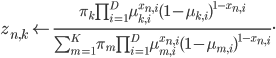
In order to update the latent variable distribution (i.e. image assignment to clusters) at the expectation step, we need to set the probability distribution of  to
to  .
.
However, we cannot calculate this distribution exactly, hence we will have to approximate this assignment. A simple way of doing it is to replace the current values of  with the expected ones:
\begin{equation} \label{eq:z}
\begin{split}
z_{n, k}^\text{new} \leftarrow \mathbb{E}_{\mathbf{Z} | \mathbf{X}, \mathbf{\mu}, \mathbf{\pi}}[z_{n, k}] &= \sum_{z_{n, k}} \,\text{Pr}(z_{n,k} | \mathbf{x_n}, \mathbf{\mu}, \mathbf{\pi}) \, z_{n,k}\\
&= \frac{\pi_k \,\text{Pr}(\mathbf{x_n} |\mathbf{\mu_k})}{\sum_{m = 1}^K \pi_m \,\text{Pr}(\mathbf{x_n} | \mathbf{\mu_m})} \\
&= \frac{\pi_k \prod_{i = 1}^D \mu_{k, i}^{x_{n, i}} (1 - \mu_{k, i})^{1 - x_{n, i}} }{\sum_{m = 1}^K \pi_m \prod_{i = 1}^D \mu_{m, i}^{x_{n, i}} (1 - \mu_{m, i})^{1 - x_{n, i}}}.
\end{split}
\end{equation}
(Notice that after this update  is no longer represented as 1-of- vector, i.e. the same image can be "partially" assigned to multiple clusters.)
In the maximization step we need to maximize the model parameters (i.e. the mixing coefficients and the pixel distributions) using the update equation from earlier
![\mathbf{\theta}^\text{new} \leftarrow \underset{\mathbf{\theta}}{\text{arg max }} \mathbb{E}_{\mathbf{Z} | \mathbf{X}, \theta^\text{old}} \left[ \mathcal{L}(\theta) \right].](http://blog.manfredas.com/wp-content/plugins/latex/cache/tex_7b765729a0303627aca0d776d313549f.gif)
Observe that
\begin{align}
\mathbb{E}_{\mathbf{Z} | \mathbf{X}, \theta^\text{old}} \left[ \mathcal{L}(\theta) \right] &= \sum_{n = 1}^N \sum_{k = 1}^K \mathbb{E}_{\mathbf{Z} | \mathbf{X}, \mathbf{\mu}^\text{old}, \mathbf{\pi}^\text{old}} \left[ z_{n, k} \right] \left( \ln \pi_k + \sum_{i = 1}^D x_{n, i} \ln \mu_{k, i} + (1 - x_{n, i}) \ln (1 - \mu_{k, i}) \right).
\end{align}
The equation above can be maximized w.r.t.  by simply setting its derivative to zero:
\begin{align}
\frac{\partial}{\partial \mu_{m, j}} \mathbb{E}_{\mathbf{Z} | \mathbf{X}, \theta^\text{old}} \left[ \mathcal{L}(\theta) \right] &= \sum_{n = 1}^N \mathbb{E}_{\mathbf{Z} | \mathbf{X}, \mathbf{\mu}^\text{old}, \mathbf{\pi}^\text{old}} \left[ z_{n, m} \right] \left( \frac{x_{n, j}}{\mu_{m, j}} - \frac{1 - x_{n, j}}{1 - \mu_{m, j}} \right) \\
&= \sum_{n = 1}^N z_{n, m}^\text{new} \frac{x_{n, j} - \mu_{m, j}}{\mu_{m, j} (1 - \mu_{m, j})} = 0 \Leftrightarrow \\
\mu_{m, j} &= \frac{1}{N_m} \sum_{n = 1}^N x_{n, j} z_{n, m}^\text{new},
\end{align}
where  is the effective number of images assigned to cluster
  .
.
Then the full cluster pixel distribution vector  can be written as

where
 is the weighted mean of the images associated with cluster .
To maximize ![\mathbb{E}_{\mathbf{Z} | \mathbf{X}, \theta^\text{old}} \left[ \mathcal{L}(\theta) \right]](http://blog.manfredas.com/wp-content/plugins/latex/cache/tex_2bdca63d7b1c6b52f12beb127b6707eb.gif) w.r.t. the mixing coefficients (subject to the constraint
w.r.t. the mixing coefficients (subject to the constraint  ) we can use the Lagrange multipliers, yielding the following optimization problem:
\begin{equation*}
\Lambda(\theta, \lambda) := \mathbb{E}_{\mathbf{Z} | \mathbf{X}, \theta^\text{old}} \left[ \mathcal{L}(\theta) \right] + \lambda \left( \sum_{k = 1}^K \pi_k - 1 \right).
\end{equation*}
The optimizing solution can then be found again with simple partial derivatives:
\begin{align}
\frac{\partial}{\partial \pi_{m}} \Lambda(\theta, \lambda) &= \frac{1}{\pi_m} \sum_{n = 1}^N z_{n,m}^\text{new} + \lambda = 0 \Leftrightarrow \\
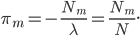
\pi_m &= -\frac{N_m}{\lambda},
\end{align}
\begin{align}
\frac{\partial}{\partial \lambda} \Lambda(\theta, \lambda) &= \sum_{k = 1}^K \pi_k - 1 = 0 \Leftrightarrow \\
\sum_{k = 1}^K \pi_k &= 1.
\end{align}
By combining these two results 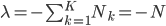 , and thus
Done!
2.3. Summary
In summary, the update equations for Bernoulli Mixture Models using E-M are:
- Expectation step:
- Maximization step:


where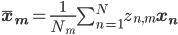 and
and  .
.
3. References
[Dempster et al, 1977] A. P. Dempster, N. M. Laird, D. B. Rubin. "Maximum Likelihood from Incomplete Data via the EM Algorithm". Journal of the Royal Statistical Society. Series B (Methodological) 39 (1): 1–38.
[Bishop, 2006] C. M. Bishop. "Pattern Recognition and Machine Learning". Springer, 2006. ISBN 9780387310732.