Even though the title is quite a mouthful, this post is about two really cool ideas:
- A solution to the "chicken-and-egg" problem (known as the Expectation-Maximization method, described by A. Dempster, N. Laird and D. Rubin in 1977), and
- An application of this solution to automatic image clustering by similarity, using Bernoulli Mixture Models.
For the curious, an implementation of the automatic image clustering is shown in the video below. The source code (C#, Windows x86/x64) is also available for download!
Automatic clustering of handwritten digits from MNIST database using Expectation-Maximization algorithm
While automatic image clustering nicely illustrates the E-M algorithm, E-M has been successfully applied in a number of other areas: I have seen it being used for word alignment in automated machine translation, valuation of derivatives in financial models, and gene expression clustering/motif finding in bioinformatics.
As a side note, the notation used in this tutorial closely matches the one used in Christopher M. Bishop's "Pattern Recognition and Machine Learning". This should hopefully encourage you to check out his great book for a broader understanding of E-M, mixture models or machine learning in general.
Alright, let's dive in!
1. Expectation-Maximization Algorithm
Imagine the following situation. You observe some data set  (e.g. a bunch of images). You hypothesize that these images are of
  different objects... but you don't know which images represent which objects.
Let  be a set of latent (hidden) variables, which tell precisely that: which images represent which objects.
Clearly, if you knew , you could group images into the clusters (where each cluster represents an object), and vice versa, if you knew the groupings you could deduce . A classical "chicken-and-egg" problem, and a perfect target for an Expectation-Maximization algorithm.
Here's a general idea of how E-M algorithm tackles it. First of all, all images are assigned to clusters arbitrarily. Then we use this assignment to modify the parameters of the clusters (e.g. we change what object is represented by that cluster) to maximize the clusters' ability to explain the data; after which we re-assign all images to the expected most-likely clusters. Wash, rinse, repeat, until the assignment explains the data well-enough (i.e. images from the same clusters are similar enough).
(Notice the words in bold in the previous paragraph: this is where the expectation and maximization stages in the E-M algorithm come from.)
To formalize (and generalize) this a bit further, say that you have a set of model parameters  (in the example above, some sort of cluster descriptions).
To solve the problem of cluster assignments we effectively need to find model parameters  that maximize the likelihood of the observed data , or, equivalently, the model parameters that maximize the log likelihod
Using some simple algebra we can show that for any latent variable distribution  , the log likelihood of the data can be decomposed as
\begin{align}
\ln \,\text{Pr}(\mathbf{X} | \theta) = \mathcal{L}(q, \theta) + \text{KL}(q || p), \label{eq:logLikelihoodDecomp}
\end{align}
where  is the Kullback-Leibler divergence between and the posterior distribution
  , and
, and
\begin{align}
\mathcal{L}(q, \theta) := \sum_{\mathbf{Z}} q(\mathbf{Z}) \left( \mathcal{L}(\theta) - \ln q(\mathbf{Z}) \right)
\end{align}
with  being the "complete-data" log likelihood (i.e. log likelihood of both observed and latent data).
To understand what the E-M algorithm does in the expectation (E) step, observe that  for any and hence
  is a lower bound on
  .
.
Then, in the E step, the gap between the and is minimized by minimizing the Kullback-Leibler divergence with respect to (while keeping the parameters  fixed).
Since is minimized at  when
when  , at the E step is set to the conditional distribution .
To maximize the model parameters in the M step, the lower bound is maximized with respect to the parameters (while keeping fixed; notice that in this equation corresponds to the old set of parameters, hence to avoid confusion let  ).
).
The function that is being maximized w.r.t. at the M step can be re-written as
\begin{align*}
\theta^\text{new} &= \underset{\mathbf{\theta}}{\text{arg max }} \left. \mathcal{L}(q, \theta) \right|_{q(\mathbf{Z}) = \,\text{Pr}(\mathbf{Z} | \mathbf{X}, \theta^\text{old})} \\
&= \underset{\mathbf{\theta}}{\text{arg max }} \left. \sum_{\mathbf{Z}} q(\mathbf{Z}) \left( \mathcal{L}(\theta) - \ln q(\mathbf{Z}) \right) \right|_{q(\mathbf{Z}) = \,\text{Pr}(\mathbf{Z} | \mathbf{X}, \theta^\text{old})} \\
&= \underset{\mathbf{\theta}}{\text{arg max }} \sum_{\mathbf{Z}} \,\text{Pr}(\mathbf{Z} | \mathbf{X}, \theta^\text{old}) \left( \mathcal{L}(\theta) - \ln \,\text{Pr}(\mathbf{Z} | \mathbf{X}, \theta^\text{old}) \right) \\
&= \underset{\mathbf{\theta}}{\text{arg max }} \mathbb{E}_{\mathbf{Z} | \mathbf{X}, \theta^\text{old}} \left[ \mathcal{L}(\theta) \right] - \sum_{\mathbf{Z}} \,\text{Pr}(\mathbf{Z} | \mathbf{X}, \theta^\text{old}) \ln \,\text{Pr}(\mathbf{Z} | \mathbf{X}, \theta^\text{old}) \\
&= \underset{\mathbf{\theta}}{\text{arg max }} \mathbb{E}_{\mathbf{Z} | \mathbf{X}, \theta^\text{old}} \left[ \mathcal{L}(\theta) \right] - (C \in \mathbb{R}) \\
&= \underset{\mathbf{\theta}}{\text{arg max }} \mathbb{E}_{\mathbf{Z} | \mathbf{X}, \theta^\text{old}} \left[ \mathcal{L}(\theta) \right],
\end{align*}
i.e. in the M step the expectation of the joint log likelihood of the complete data is maximized with respect to the parameters .
So, just to summarize,
- Expectation step:
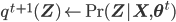
- Maximization step:
![\mathbf{\theta}^{t + 1} \leftarrow \underset{\mathbf{\theta}}{\text{arg max }} \mathbb{E}_{\mathbf{Z} | \mathbf{X}, \theta^\text{t}} \left[ \mathcal{L}(\theta) \right]](http://blog.manfredas.com/wp-content/plugins/latex/cache/tex_ce39f6d35750f5ced3727687ba5d72c3.gif) (where superscript
(where superscript  indicates the value of parameter at time
  ).
).
Phew. Let's go to the image clustering example, and see how all of this actually works. Continue reading


")