
The PhD thesis of Paul J. Werbos at Harvard in 1974 described backpropagation as a method of teaching feed-forward artificial neural networks (ANNs). In the words of Wikipedia, it lead to a "rennaisance" in the ANN research in 1980s.
As we will see later, it is an extremely straightforward technique, yet most of the tutorials online seem to skip a fair amount of details. Here's a simple (yet still thorough and mathematical) tutorial of how backpropagation works from the ground-up; together with a couple of example applets. Feel free to play with them (and watch the videos) to get a better understanding of the methods described below!
Training a single perceptron
Training a multilayer neural network
1. Background
To start with, imagine that you have gathered some empirical data relevant to the situation that you are trying to predict - be it fluctuations in the stock market, chances that a tumour is benign, likelihood that the picture that you are seeing is a face or (like in the applets above) the coordinates of red and blue points.
We will call this data training examples and we will describe  th training example as a tuple
  , where
  is a vector of inputs and
  is the observed output.
Ideally, our neural network should output  when given
  as an input. In case that does not always happen, let's define the error measure as a simple squared distance between the actual observed output and the prediction of the neural network:
 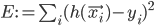 , where
  is the output of the network.
2. Perceptrons (building-blocks)
The simplest classifiers out of which we will build our neural network are perceptrons (fancy name thanks to Frank Rosenblatt). In reality, a perceptron is a plain-vanilla linear classifier which takes a number of inputs  , scales them using some weights
  , adds them all up (together with some bias
  ) and feeds everything through an activation function
  .
.
A picture is worth a thousand equations:
Perceptron (linear classifier)")
To slightly simplify the equations, define  and
and  . Then the behaviour of the perceptron can be described as
  , where
  and
and  .
.
To complete our definition, here are a few examples of typical activation functions:
- sigmoid:
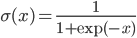 ,
, - hyperbolic tangent:
 ,
, - plain linear
 and so on.
Now we can finally start building neural networks. Continue reading

