
The PhD thesis of Paul J. Werbos at Harvard in 1974 described backpropagation as a method of teaching feed-forward artificial neural networks (ANNs). In the words of Wikipedia, it lead to a "rennaisance" in the ANN research in 1980s.
As we will see later, it is an extremely straightforward technique, yet most of the tutorials online seem to skip a fair amount of details. Here's a simple (yet still thorough and mathematical) tutorial of how backpropagation works from the ground-up; together with a couple of example applets. Feel free to play with them (and watch the videos) to get a better understanding of the methods described below!
Training a single perceptron
Training a multilayer neural network
1. Background
To start with, imagine that you have gathered some empirical data relevant to the situation that you are trying to predict - be it fluctuations in the stock market, chances that a tumour is benign, likelihood that the picture that you are seeing is a face or (like in the applets above) the coordinates of red and blue points.
We will call this data training examples and we will describe  th training example as a tuple
  , where
  is a vector of inputs and
  is the observed output.
Ideally, our neural network should output  when given
  as an input. In case that does not always happen, let's define the error measure as a simple squared distance between the actual observed output and the prediction of the neural network:
 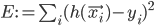 , where
  is the output of the network.
2. Perceptrons (building-blocks)
The simplest classifiers out of which we will build our neural network are perceptrons (fancy name thanks to Frank Rosenblatt). In reality, a perceptron is a plain-vanilla linear classifier which takes a number of inputs  , scales them using some weights
  , adds them all up (together with some bias
  ) and feeds everything through an activation function
  .
.
A picture is worth a thousand equations:
Perceptron (linear classifier)")
To slightly simplify the equations, define  and
and  . Then the behaviour of the perceptron can be described as
  , where
 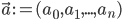 and
and 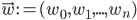 .
.
To complete our definition, here are a few examples of typical activation functions:
- sigmoid:
 ,
, - hyperbolic tangent:
 ,
, - plain linear
 and so on.
Now we can finally start building neural networks. The simplest kind of network that we can build is... exactly, one perceptron! Here's how we can train it to classify things!
3. Single-layer neural network
We defined the error earlier as . Obviously, since we are using a single perceptron both our error and the output of the network (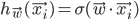 ) depend on the weights vector
  .
.
Incorporating those observations into the updated error measure we obtain 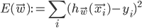 .
.
Our goal is to find such a vector of weights that  is minimised - that way our perceptron will correctly predict the output for all inputs of our training examples!
We will do that by applying the gradient descent algorithm: in essence we will treat the error as a surface in n-dimensional space, then we will find a greatest downwards slope at the current point  and will go in that direction to obtain
  . This way hopefully we will find a minimum point on the error surface and we will use the coordinates of that point as the final weight vector.
By skipping a great deal of maths on whether the minimum point exists, is it unique and global, can we "overjump" it by accident, what are the conditions for the following partial derivatives to exist, etc, etc; we will dive straight in hoping for the best and will calculate the gradient of the error surface at . Then we will take a step in the opposite direction of the gradient (i.e. in the direction of the fastest decreasing slope on the error surface) to obtain  .
.
To express it in a slightly more mathematical way, we will start with some randomized (!) weight vector  and will train our perceptron by updating the weights
\begin{align} \vec{w}_{t+1} := \vec{w_t} - \eta \frac{\partial E(\vec{w})}{\partial \vec{w}} \bigg|_{\vec{w_t}}, \end{align}
where  is known as a learning rate (a simple scaling factor that typically ranges between zero and one).
Observe that
\begin{align} \frac{\partial E(\vec{w})}{\partial \vec{w}} = \left( \frac{\partial E(\vec{w})}{\partial w_0},\frac{\partial E(\vec{w})}{\partial w_1}, ... ,\frac{\partial E(\vec{w})}{w_n} \right), \end{align}
and we can calculate
\begin{align} \frac{\partial E(\vec{w})}{\partial w_j} &= \frac{\partial}{\partial w_j} \sum_i (h_{\vec{w}}(\vec{x_i}) - y_i)^2 \\ &= \sum_i 2(h_{\vec{w}}(\vec{x_i}) - y_i) \frac{\partial}{\partial w_j} (h_{\vec{w}}(\vec{x_i}) - y_i) \\ &= \sum_i 2(h_{\vec{w}}(\vec{x_i}) - y_i) \frac{\partial}{\partial w_j} \sigma(\vec{x_i} \cdot \vec{w}) \\ &= \sum_i 2(h_{\vec{w}}(\vec{x_i}) - y_i) \; \sigma ' (\vec{x_i} \cdot \vec{w}) \frac{d}{d w_j} \vec{x_i} \cdot \vec{w} \\ &= \sum_i 2(h_{\vec{w}}(\vec{x_i}) - y_i) \; \sigma ' (\vec{x_i} \cdot \vec{w}) \frac{d}{d w_j} \sum_{k=1}^n x_{i,k} w_k \\ &= 2 \sum_i (h_{\vec{w}}(\vec{x_i}) - y_i) \; \sigma ' (\vec{x_i} \cdot \vec{w}) x_{i,j} \end{align}
for each  .
.
3.1. Example single-layer neural network
In this applet, a perceptron takes two inputs (normalized x and y coordinates  and
and  , i.e.
  ,
,  ) and uses sigmoid as an activation function with the learning rate
  .
.
Then, using a previous general result
\begin{align} \frac{\partial E(\vec{w})}{\partial w_j} &= 2 \sum_i (h_{\vec{w}}(\vec{x_i}) - y_i) \; \sigma ' (\vec{x_i} \cdot \vec{w}) x_{i,j} \\ &= 2 \sum_i (\sigma(\vec{w} \cdot \vec{x_i}) - y_i) \sigma(\vec{x_i} \cdot \vec{w}) (1 - \sigma(\vec{x_i} \cdot \vec{w})) x_{i,j}, \end{align}
(since for the sigmoid activation function  ); and thus
\begin{align} \frac{\partial E(\vec{w})}{\partial \vec{w}} = 2 \sum_i (\sigma(\vec{w} \cdot \vec{x_i}) - y_i) \sigma(\vec{x_i} \cdot \vec{w}) (1 - \sigma(\vec{x_i} \cdot \vec{w})) \vec{x_i}. \end{align}
The final algorithm to update the weight vector  (which is initially randomized) then is
\begin{align} \vec{w}_{t+1} := \vec{w_t} - 0.2 \sum_i (h_{\vec{w}_t}(\vec{x_i}) - y_i) h_{\vec{w}_t}(\vec{x_i}) (1 - h_{\vec{w}_t}(\vec{x_i})) \vec{x_i}, \end{align}
where  .
.
However, a single perceptron is extremely limited in the sense that different classes of examples must be separable with a hyperplane (hence the name, linear classifier), which is usually not the case in real-life applications.
Time to bump things up a notch: let's connect a few of them together to obtain a multilayer feed-forward neural network!
4. Multilayer neural network
Let's consider a general case first: a completely unrestricted feed-forward structure (with the only condition being that there are no loops between the perceptrons to avoid general madness and chaos).
Since it is structurally more complex than just a single perceptron, take a look at the following figure that explains some more notation:
Multilayer neural network
Here the weight  connects perceptrons and
  , the sum of the weighed inputs of perceptron is denoted by
  where
where  iterates over all perceptrons connected to , and the output of is written as
  , where
  is 's activation function.
We will use the same error measure , except now the weights vector will contain all the weights in the network, i.e.  for all
  .
.
To find that minimizes using gradient descent we have to calculate  (again). However, this time it is (very slightly) more involved.
First of all let's separate the contributions of individual training examples to the overall error using the following observation:
\begin{align} \frac{\partial E(\vec{w})}{\partial \vec{w}} = \sum_i \frac{\partial E_i(\vec{w})}{\partial \vec{w}}, \end{align}
where  .
.
Then
\begin{align} \frac{\partial E_i(\vec{w})}{\partial w_{j \rightarrow k}} &= \frac{\partial}{\partial w_{j \rightarrow k}} (h_{\vec{w}}(\vec{x_i}) - y_i)^2 \\ &= 2 (h_{\vec{w}}(\vec{x_i}) - y_i) \frac{\partial h_{\vec{w}}(\vec{x_i})}{\partial w_{j \rightarrow k}} \\ &= 2 (h_{\vec{w}}(\vec{x_i}) - y_i) \frac{\partial h_{\vec{w}}(\vec{x_i})}{\partial s_k} \frac{\partial s_k}{\partial w_{j \rightarrow k}} \\ &= 2 (h_{\vec{w}}(\vec{x_i}) - y_i) \frac{\partial h_{\vec{w}}(\vec{x_i})}{\partial s_k} z_j. \end{align}
If is an output node, then
\begin{align} \frac{\partial h_{\vec{w}}(\vec{x_i})}{\partial s_k} = \frac{d \sigma(s_k)}{d s_k} = \sigma' (s_k)\end{align}
and thus
\begin{align} \frac{\partial E_i(\vec{w})}{\partial w_{j \rightarrow k}} &= 2 (h_{\vec{w}}(\vec{x_i}) - y_i) \; \sigma ' (s_k)\; z_j. \end{align}
However, if is not an output node, then a change in  can affect all the nodes which are connected to 's output, i.e.
\begin{align} \frac{\partial h_{\vec{w}}(\vec{x_i})}{\partial s_k} &= \frac{\partial h_{\vec{w}}(\vec{x_i})}{\partial z_k} \frac{\partial z_k}{\partial s_k} \\ &= \frac{\partial h_{\vec{w}}(\vec{x_i})}{\partial z_k} \sigma ' (s_k) \\ &= \sum_{o \in \{ v \; | \; v \text{ is connected to } k \}} \frac{\partial h_{\vec{w}}(\vec{x_i})}{\partial s_o} \frac{\partial s_o}{\partial z_k} \sigma ' (s_k) \\ &= \sum_{o \in \{ v \; | \; v \text{ is connected to } k \}} \frac{\partial h_{\vec{w}}(\vec{x_i})}{\partial s_o} w_{k \rightarrow o} \; \sigma ' (s_k), \end{align}
... and we are almost done! All what is left to do is to place the th example at the inputs of our neural network, calculate and  for all the nodes (the forward-propagation step) and work our way backwards from the output node calculating
  (hence the name, backpropagation).
To summarize, if is an output node, then
\begin{align} \frac{\partial E_i(\vec{w})}{\partial w_{j \rightarrow k}} &= 2 (h_{\vec{w}}(\vec{x_i}) - y_i) \; \sigma ' (s_k)\; z_j, \end{align}
otherwise
\begin{align} \frac{\partial E_i(\vec{w})}{\partial w_{j \rightarrow k}} &= 2 (h_{\vec{w}}(\vec{x_i}) - y_i) \; \sigma ' (s_k)\; z_j \sum_{o \in \{ v \; | \; v \text{ conn. to } k \}} \frac{\partial h_{\vec{w}}(\vec{x_i})}{\partial s_o} w_{k \rightarrow o}. \end{align}
Then after the following is obtained
\begin{align} \frac{\partial E_i(\vec{w})}{\partial \vec{w}} = \left( \; \; \frac{\partial E_i(\vec{w})}{\partial w_{j \rightarrow k}} \; \; \right), \forall j, k \end{align}
the weight vector can either be updated in one go (batch update)
\begin{align} \vec{w}_{t+1} := \vec{w_t} - \eta \frac{\partial E(\vec{w})}{\partial \vec{w}} \bigg|_{\vec{w_t}} = \vec{w_t} - \eta \sum_i \frac{\partial E_i(\vec{w})}{\partial \vec{w}}\bigg|_{\vec{w_t}}, \end{align}
or it can be updated sequentially using one training example at a time:
\begin{align} \vec{w}_{t+1} := \vec{w_t} - \eta \frac{\partial E_i(\vec{w})}{\partial \vec{w}} \bigg|_{\vec{w_t}}.\end{align}
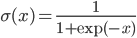
4.1. Example multilayer network
If you launch and play with the applet above, you will see that it is able to separate classes non-linearly (indicating that it's using more than one perceptron). It is built using this two-layer neural network:
Two-layer neural network example
The weights vector contains all the weights in the network, i.e.
\begin{align} \vec{w} = ( w_{in_1 \rightarrow 1}, w_{in_x \rightarrow 1}, w_{in_y \rightarrow 1}, w_{in_1 \rightarrow 2}, ..., w_{in_y \rightarrow 5}, w_{in_1 \rightarrow 6}, w_{1 \rightarrow 6}, w_{2 \rightarrow 6}, ..., w_{5 \rightarrow 6}). \end{align}
Each perceptron is using sigmoid as its activation function and the output of the perceptron  is the output for the whole network, i.e.
  .
.
Then an individual point i (with x and y coordinates normalized) is considered as an th training example and fed through the network. While it's being propagated, each  and
and  for
for  are stored.
Then the gradient of an th error surface is calculated as follows:
\begin{align}
\frac{\partial E_i(\vec{w})}{\partial \vec{w}} &= \left( \frac{\partial E_i(\vec{w})}{\partial w_{in_1 \rightarrow 1}},\frac{\partial E_i(\vec{w})}{\partial w_{in_x \rightarrow 1}}, ..., \frac{\partial E_i(\vec{w})}{\partial w_{in_y \rightarrow 5}},\frac{\partial E_i(\vec{w})}{\partial w_{in_1 \rightarrow 6}},\frac{\partial E_i(\vec{w})}{\partial w_{1 \rightarrow 6}},\frac{\partial E_i(\vec{w})}{\partial w_{2 \rightarrow 6}}, ..., \frac{\partial E_i(\vec{w})}{\partial w_{5 \rightarrow 6}} \right) , \end{align}
where
\begin{align} \frac{\partial E_i(\vec{w})}{\partial w_{in_1 \rightarrow 1}} &= 2 (h_{\vec{w}}(\vec{x_i}) - y_i) \; \sigma ' (s_1)\; \frac{\partial h_{\vec{w}}(\vec{x_i})}{\partial s_6} w_{1 \rightarrow 6} \\
&= 2 (z_6 - y_i) \; \sigma (s_1) \; (1 - \sigma (s_1)) \; \sigma (s_6) \; (1 - \sigma (s_6)) \; w_{1 \rightarrow 6}, \\
\frac{\partial E_i(\vec{w})}{\partial w_{in_x \rightarrow 1}} &= 2 (z_6 - y_i) \; \sigma (s_1) \; (1 - \sigma (s_1)) \; {in}_x \; \sigma (s_6) \; (1 - \sigma (s_6)) \; w_{1 \rightarrow 6}, \\
& \vdots \\
\frac{\partial E_i(\vec{w})}{\partial w_{in_y \rightarrow 5}} &= 2 (z_6 - y_i) \; \sigma (s_5) \; (1 - \sigma (s_5)) \; {in}_y \; \sigma (s_6) \; (1 - \sigma (s_6)) \; w_{5 \rightarrow 6}, \\
\frac{\partial E_i(\vec{w})}{\partial w_{in_1 \rightarrow 6}} &= 2 (h_{\vec{w}}(\vec{x_i}) - y_i) \; \sigma ' (s_6) \\
&= 2 (z_6 - y_i) \; \sigma (s_6) \; (1 - \sigma (s_6)) , \\
\frac{\partial E_i(\vec{w})}{\partial w_{1 \rightarrow 6}} &= 2 (z_6 - y_i) \; \sigma (s_6) \; (1 - \sigma (s_6)) \; z_1, \\
\frac{\partial E_i(\vec{w})}{\partial w_{2 \rightarrow 6}} &= 2 (z_6 - y_i) \; \sigma (s_6) \; (1 - \sigma (s_6)) \; z_2, \\
& \vdots \\
\frac{\partial E_i(\vec{w})}{\partial w_{5 \rightarrow 6}} &= 2 (z_6 - y_i) \; \sigma (s_6) \; (1 - \sigma (s_6)) \; z_5.
\end{align}
Finally, the network is sequentially trained with the learning rate  (starting with a random initial weight vector
  )
)
\begin{align} \vec{w}_{t+1} := \vec{w_t} - 0.5 \frac{\partial E_i(\vec{w})}{\partial \vec{w}} \bigg|_{\vec{w_t}}.\end{align}
That's it, I hope it sheds some light on the backpropagation!
Great post, this is very similar to SNN (Sharky Neural Network), see: http://sharktime.com/us_SharkyNeuralNetwork.html
Thanks for the great tutorial! Most references miss exactly this part between "this is a neuron, and this is Boltzmann recurrent neural network".
http://9gag.com/gag/4614736
Thanks, Gmaz!
Nice post and nice applets!
I am curious about the interpretation of the plots of your applets. If I understand correctly class 1 (e.g. red) corresponds to :
z6 = 0 (or abs(z6) < eps)
and class 2 (e.g. blue) corresponds to:
z6 = 1 (or abs(z6-1) < eps)
where eps is a 'small' number.
And then for the plots you create a mesh grid with (x_1 , x_2 ) pairs , perform forward propagation for each pair and the color corresponds to the activation level of z6 (e.g. red being 0 blue being 1 and the rest sth in between?)If that's the case I am amazed because it seems to be deadly fast!
Great, Thanks.
Hi, I was wondering how you made your NN figures? They look really slick. And great tutorial.
Thanks, J-dog. The figures were made using Inkscape (free and open-source).